Stability Analysis
Two important questions in the investigation of cardiac arrhythmias are how these activation patterns develop and how their complexity can be characterized. What properties of the tissue determine its susceptibility to arrhythmias? Where and when are certain activation patterns most sensitive to perturbations? What makes irregular activity easy or difficult to terminate? We expect that the answers will yield valuable information for the prevention of arrhythmias and about strategies to terminate them. One of our approaches to tackle these questions is to view cardiac tissue as a high-dimensional non-linear dynamical system. Using a number of different numerical models of cardiac tissue, we carry out linear stability analysis of different activation patterns to assess their (ir)regularity. As a very general method that can be applied to arbitrary attractors of the system, this procedure yields growth rates (so-called Lyapunov exponents) of perturbations localized at specific sensitive spots (given by Lyapunov vectors) and allows us to estimate the attractor dimension – a quantitative measure for the complexity of the dynamics. Abrupt changes of excitation patterns (Fig. 1) and symmetries in the system can be detected as well as the onset of chaotic activity.
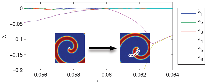
Figure 1 Detection of bifurcations via Lyapunov exponents. The bifurcation parameter ε is a model parameter, which turns a rigidly rotating spiral wave (left) into a meandering spiral (right). Transitions between qualitatively different activation patterns (bifurcations) are indicated by one or more Lyapunov exponents becoming zero, which is the case at ε≈0.06 here. Lyapunov exponents (i.e. growth rates of perturbation modes) are ordered by size, with λ1 being the largest. All Lyapunov exponents are less or equal to zero, since both the rigidly rotating spiral wave and the meandering spiral wave are stable activation patterns.
In extended media instabilities often occur first locally and then grow and spread out. Such scenarios can be investigated and characterized by means of Lyapunov vectors. For spatio-temporal systems Lyapunov vectors are given as patterns evolving in time and may thus be interpreted as generalizations of the concept of (active) modes [1]. In state space (more precisely, in the tangent space of the state space) Lyapunov vectors point in the directions of characteristic growth of perturbations (on average quantified by Lyapunov exponents). Usually two types of “Lyapunov vectors” have to be distinguished: (i) the orthogonal set of vectors occurring with the standard algorithm for computing Lyapunov exponents (based on QR-decomposition or Gram-Schmidt reorthogonalisation) and (ii) so-called covariant Lyapunov vectors, that are not orthogonal but possess several desirable (invariant) features. Covariant Lyapunov vectors became practically available only recently due to novel numerical algorithms proposed by Ginelli et al. [2] and Wolfe and Samuelson [3]. With a view to applications to excitable media we prepared a detailed study of the theory and computation of covariant Lyapunov vectors including new alternatives for their efficient computation [4].
In order to transfer the knowledge we gain about the nature of certain instabilities to experiments, the next step will be to connect these rather abstract measures to quantities that can be measured in real cardiac tissue, e.g., the number of phase singularities or the propagation velocity. Preliminary results show that there is a close connection between the complexity of spatio-temporal chaos and the number of rotating waves. Another focus is on the relationship between the stability of wave patterns and the degree of cellular heterogeneity (e.g., fibrotic tissue).
References
- P.V. Kuptsov and U. Parlitz, Phys. Rev. E 81, 036214 (2010).
- F. Ginelli et al., Phys. Rev. Lett. 99, 130601 (2007).
- C.L. Wolfe and R.M. Samuelson, Tellus 59A, 355-366 (2007).
- P.V. Kuptsov and U. Parlitz, (submitted for publication).