State and Parameter Estimation
While physical models often can be derived from first principles, they may contain parameters whose values are not or only partially known and may depend on the physical context. To identify these parameters, the model may be adapted to experimental data. Here both (unknown) parameters and model variables have to be adjusted, including hidden (i.e. not observed) state variables determining the temporal evolution of the model. For some applications this adaption has to be continuously updated to “track” some process by continously incorporating measured data into the model (a procedure called data assimilation in geosciences and meteorology). To accomplish the task of parameter estimation we employ synchronization and nonlinear optimization methods. With the synchronization approach [1] the available time series is used to drive a simulation model in order to achieve (generalized) synchronization. The synchronization error depends on the model parameters and attains a global minimum if they coincide with the “true” values holding for the experimental system. As an advantage of this approach all (unobserved) state variables approach their true values due to synchronization and have not to be explicitly estimated.
As an example for synchronization based data assimilation we developed a scheme for synchronizing extended excitable media [2]. Similar to possible experimental situations we assume that time series are sampled at sensors providing local (spatial) averages of the measured variable. Multivariate time series from different sensors are then fed into the model to synchronize it with the observed dynamics. Relevant parameters of this synchronization scheme are the sensors’ size and (mutual) distance and the coupling strength. This is demonstrated using a generic model of excitable media exhibiting spiral wave dynamics and chaotic spiral break-up. The system generating the data and the adapted “model” are both implemented on a graphics processing unit (GPU) providing a speedup factor of 50 - 100 compared to a conventional CPU [2,3]. Fig. 1A shows two snapshots of the synchronization process for chaotic dynamics generated by a (cubic) Barkley-model. The synchronization error landscape shown in Fig. 1B can be used to identify the correct model parameters corresponding to the (global) minimum.
Figure 1
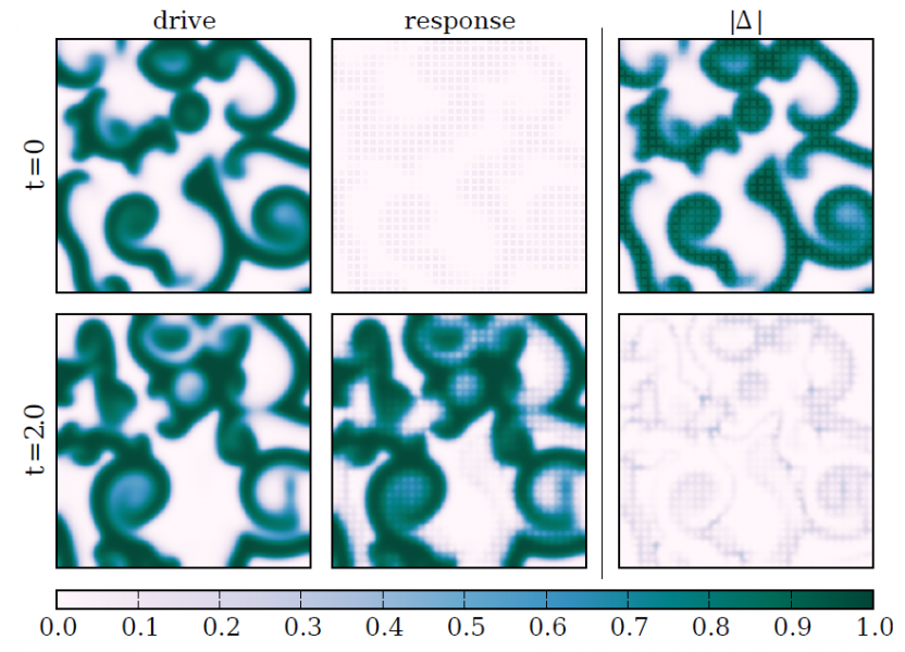
Synchronization-based state and parameter estimation of a chaotic 2D Barkley model ($a=-0.75$, $b=0.06$, $ε=1/12$).
(A) Snapshots of the solution of the driving and response systems as well as their differences are plotted in columns 1-3, respectively. The first row shows conditions at $t=0$, i.e. when coupling is applied. The socond row shows solution at $t=2$, when synchronization has almost been reached.
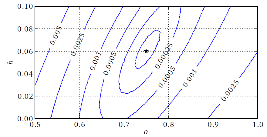
(B) Contours showing the Euklidean norm of the synchronization error if the parameters a and b of the Barkley model of the response system do not match those of the driving system. The star indicates the minimum of the synchronization error.
Optimization based methods aim at reproducing the observed time series by means of the corresponding model output, too. However, since no synchronization is employed, one additionally has to make sure that the underlying temporal evolution of the state variables fits to the model dynamics. This can be achieved by imposing the dynamical equations as constraints on the optimization process [4] or by including (deviations from) the dynamical equations in the cost function [5]. We use and evaluate both optimization approaches. An example for the second method is shown in Fig. 3, using the Hindmarsh-Rose (HR) neuron model [5], where the adapted model output (solid blue line) has been fitted to the data. Despite the two time scales in the observed signal and the superimposed measurement noise the implemented parameter estimation algorithm is able to recover the correct values of four system parameters and the dynamics of the (slow) “hidden” variables. We also succeeded in identifying hyperchaotic dynamics (dimension > 8) and system parameters of a generalized Rössler system [5] from a scalar time series and parameters of cardiac cell models [6], which indicates the enormous potential of the optimization method.
Figure 2
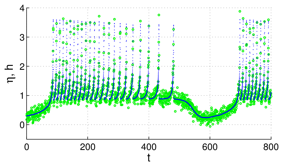
Optimization-based state and parameter estimation of a chaotic Hindemarsh-Rose neuron model. The time series generated by the model (blue dots) was adapted to the observed time series (green circles) (from [4]).
In general, an important topic and task is the detection of parameter redundancies that (may) occur if many model parameters are unknown (as is the case, for example, in cardiac cell models). In such a case the true parameter values may be not observable, i.e. different combinations of model parameters provide the same output (compared with the observed time series) [6].
References
- U. Parlitz, L. Junge and L. Kocarev, Phys. Rev. E 54, 6253-6529 (1996).
- S. Berg, P. Bittihn, S. Luther, U. Parlitz, Proceedings of the 6th ESGCO 2010, April 12-14, 2010, Berlin, Germany.
- S. Berg, S. Luther, and U. Parlitz, Chaos (to appear).
- H.D.I. Abarbanel, D. R. Creveling, R. Farsian, and M. Kostuk, SIAM J. Appl. Dyn. Syst. 8, 1341-1381 (2009).
- J. Schumann-Bischoff and U. Parlitz (submitted for publication).
- J. Schumann-Bischoff, J. Schröder-Schetelig, S. Luther, and U. Parlitz, Proceedings of the International Biosignal Processing Conference. Berlin, Germany, 2010: 097: 1-4.